
ВИЗУАЛИЗАЦИЯ ДАННЫХ
Финальный проект
Цель проекта — провести анализ динамики выбросов CO₂ и связанных социально-экономических факторов на основе открытого табличного датасета (CSV) и представить результаты в виде набора визуализаций с единым стилем оформления.
Данные и источник
Использован набор данных «CO₂ and Greenhouse Gas Emissions» от Our World in Data (OWID). Датасет распространяется в формате CSV и содержит показатели по странам и годам, включая CO₂, CO₂ на душу населения, ВВП, население и энергетические метрики. Источник (страница датасета): https://ourworldindata.org/co2-and-greenhouse-gas-emissions CSV (репозиторий OWID): https://github.com/owid/co2-data
Подготовка и обработка данных
Обработка выполнена в Python с использованием pandas. Основные шаги: • загрузка CSV; • отбор необходимых столбцов и удаление строк без ключевых полей; • формирование набора «focus» для сравнения (World, EU, Latvia, Russia, USA, China, India); • приведение типов и обработка пропусков; • расчет дополнительных показателей (например, GDP per capita = gdp / population).
Примененные статистические методы
В проекте применены следующие методы:
- Описательная статистика (describe) для понимания распределения выбросов.
- Сглаживание тренда: скользящее среднее за 10 лет для глобального ряда (World).
- Корреляционный анализ (Пирсон) для набора метрик (co2_per_capita, gdp, energy_per_capita) за последние годы.
- Визуальная проверка связи CO₂ на душу населения и GDP per capita с логарифмической шкалой по доходу.
Визуализации
Ниже приведены 4 графика разных типов (line/bar/scatter/heatmap), оформленные в едином стиле. Каждый график снабжен подписью и предназначен для поддержки интерпретации результатов.
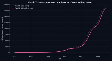
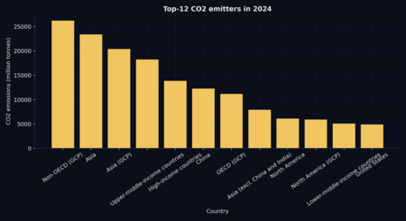
Рис. 1. Динамика глобальных выбросов CO₂: исходный ряд и 10-летнее сглаживание. Рис. 2. Топ-12 стран по объему выбросов CO₂ в последнем доступном году датасета.
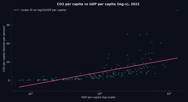
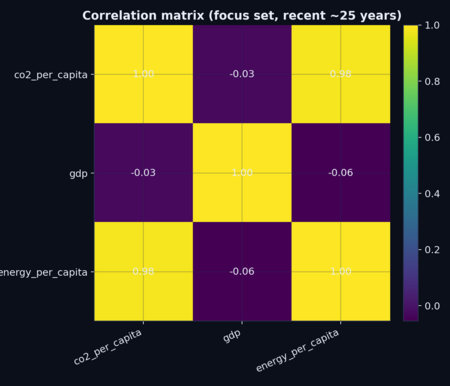
Рис. 3. Связь CO₂ на душу населения и GDP per capita (логарифмическая шкала по X) в последнем году. Рис. 4. Корреляционная матрица (Пирсон) для выбранных метрик за последние годы.
Краткие выводы
- Глобальный тренд по CO₂ демонстрирует выраженную долгосрочную динамику, которую удобнее интерпретировать после сглаживания скользящим средним.
- Вклад отдельных стран в суммарные выбросы существенно различается, что видно на столбчатой диаграмме топ-эмитентов.
- На уровне стран наблюдается нелинейная связь между уровнем дохода (GDP per capita) и CO₂ на душу населения, поэтому для визуального анализа применена логарифмическая шкала по оси X.
- Корреляционная матрица помогает оценить совместную изменчивость метрик и выбрать направления для дальнейшего анализа.
Применение генеративной модели
В процессе подготовки черновой структуры отчета и базового шаблона кода использовались автоматизированные инструменты генерации текста. Итоговые расчеты, выбор метрик, построение графиков и формулировка выводов были проверены и доработаны вручную. Модель: ChatGPT (OpenAI). Страница продукта: https://chatgpt.com/
Приложение A. Полный код (Python)
co2_owid_analysis.py
Репликация графиков и расчётов для отчёта по глобальным выбросам CO2 (OWID)
from future import annotations
import os from pathlib import Path
import numpy as np import pandas as pd import matplotlib.pyplot as plt
---------------------------
0) Конфигурация и единый стиль
---------------------------
DATA_URL = «https://raw.githubusercontent.com/owid/co2-data/master/owid-co2-data.csv" DATA_LOCAL = Path («owid-co2-data.csv») FIG_DIR = Path («figs») FIG_DIR.mkdir (parents=True, exist_ok=True)
BG = «#0B0F1A» FG = «#E8EEF7» GRID = «#2A3552» ACC1 = «#7CDBD5» ACC2 = «#FF4D8D» ACC3 = «#FFD166»
plt.rcParams.update ({ «figure.facecolor»: BG, «axes.facecolor»: BG, «savefig.facecolor»: BG, «text.color»: FG, «axes.labelcolor»: FG, «xtick.color»: FG, «ytick.color»: FG, «axes.edgecolor»: GRID, «grid.color»: GRID, «grid.alpha»: 0.35, «axes.grid»: True, «axes.titleweight»: «bold», «font.size»: 11, «font.family»: «DejaVu Sans», })
def prettify (ax: plt.Axes) -> plt.Axes: ax.spines[«top»].set_visible (False) ax.spines[«right»].set_visible (False) ax.grid (True, which="major», linewidth=0.8) ax.set_axisbelow (True) return ax
---------------------------
1) Загрузка данных
---------------------------
def load_data () -> pd.DataFrame: if DATA_LOCAL.exists (): return pd.read_csv (DATA_LOCAL) df = pd.read_csv (DATA_URL) df.to_csv (DATA_LOCAL, index=False) return df
df = load_data ()
Базовые метрики набора
years = (int (df[«year»].min ()), int (df[«year»].max ())) entities = int (df[«country»].nunique ()) rows, cols = df.shape
---------------------------
2) Фильтры и подготовка выборок
---------------------------
Страны: iso_code длиной 3 (исключаем агрегаты OWID/континенты/группы дохода)
is_country = df[«iso_code»].notna () & (df[«iso_code»].astype (str).str.len () == 3)
last_year = int (df[«year»].max ()) top12 = ( df[is_country & (df[«year»] == last_year)][[«country», «co2»]] .dropna () ) top12 = top12[top12[«co2»] > 0].sort_values («co2», ascending=False).head (12)
focus = [«World», «European Union (27)», «Latvia», «Russia», «United States», «China», «India»] recent = df[df[«country»].isin (focus) & (df[«year»] >= (last_year — 25))].copy ()
---------------------------
3) Статистические методы
---------------------------
3.1 Сглаживание (10-летнее скользящее среднее) для World CO2
world = df[df[«country»] == «World»].sort_values («year»).copy () world[«co2_roll10»] = world[«co2»].rolling (10, min_periods=5).mean ()
3.2 Корреляции (Пирсон) по выбранному фокус-набору, последние ~25 лет
corr_cols = [«co2_per_capita», «gdp», «energy_per_capita»] corr = recent[corr_cols].corr (method="pearson»)
3.3 Линейная аппроксимация CO2 per capita ~ log10(GDP per capita)
sc = df[is_country].copy () sc = sc.dropna (subset=[«gdp», «population», «co2_per_capita»]) sc = sc[sc[«population»] > 0] sc[«gdp_per_capita»] = sc[«gdp»] / sc[«population»] sc = sc.replace ([np.inf, -np.inf], np.nan).dropna (subset=[«gdp_per_capita»])
last_year_gdp = int (sc[«year»].max ()) sc = sc[sc[«year»] == last_year_gdp].copy ()
x = sc[«gdp_per_capita»].to_numpy () y = sc[«co2_per_capita»].to_numpy () lx = np.log10(x)
y = a + b*log10(x)
b, a = np.polyfit (lx, y, deg=1)
---------------------------
4) Визуализация (4 разных типа графиков)
---------------------------
4.1 Line: World CO2 + rolling mean
fig, ax = plt.subplots (figsize=(11, 6)) ax.plot (world[«year»], world[«co2»], linewidth=1.4, alpha=0.35, color=ACC1, label="World: CO2 (raw)») ax.plot (world[«year»], world[«co2_roll10»], linewidth=2.8, color=ACC2, label="World: 10y rolling mean») ax.set_title («World CO2 emissions over time (raw vs 10-year rolling mean)») ax.set_xlabel («Year») ax.set_ylabel («CO2 emissions (million tonnes)») prettify (ax) ax.legend (frameon=False) fig.tight_layout () fig.savefig (FIG_DIR / «fig1_world_co2_trend.png», dpi=200) plt.close (fig)
4.2 Bar: Top-12 emitters (последний год)
fig, ax = plt.subplots (figsize=(11, 6)) ax.bar (top12[«country»], top12[«co2»], color=ACC3, alpha=0.95) ax.set_title (f"Top-12 countries by CO2 emissions in {last_year}») ax.set_xlabel («Country») ax.set_ylabel («CO2 emissions (million tonnes)») ax.tick_params (axis="x», rotation=35) prettify (ax) fig.tight_layout () fig.savefig (FIG_DIR / «fig2_top_emitters_bar.png», dpi=200) plt.close (fig)
4.3 Scatter + regression: CO2 per capita vs GDP per capita (log-x)
fig, ax = plt.subplots (figsize=(11, 6)) ax.scatter (sc[«gdp_per_capita»], sc[«co2_per_capita»], s=14, alpha=0.25, color=ACC1) ax.set_xscale («log») xs = np.logspace (np.log10(sc[«gdp_per_capita»].min ()), np.log10(sc[«gdp_per_capita»].max ()), 200) ys = a + b * np.log10(xs) ax.plot (xs, ys, linewidth=2.0, color=ACC2, label="Linear fit on log10(GDP per capita)») ax.set_title (f"CO2 per capita vs GDP per capita (log-x), {last_year_gdp}») ax.set_xlabel («GDP per capita (log scale)») ax.set_ylabel («CO2 per capita (tonnes per person)») prettify (ax) ax.legend (frameon=False) fig.tight_layout () fig.savefig (FIG_DIR / «fig3_scatter_gdp_co2pc.png», dpi=200) plt.close (fig)
4.4 Heatmap: Correlation matrix
fig, ax = plt.subplots (figsize=(7.4, 6.2)) im = ax.imshow (corr.values, interpolation="nearest») ax.set_title («Correlation matrix (focus set, recent ~25 years)») ax.set_xticks (range (len (corr.columns)), corr.columns, rotation=25, ha="right») ax.set_yticks (range (len (corr.index)), corr.index) for i in range (corr.shape[0]): for j in range (corr.shape[1]): ax.text (j, i, f"{corr.values[i, j]:.2f}», ha="center», va="center», color=FG) prettify (ax) plt.colorbar (im, ax=ax, fraction=0.046, pad=0.04) fig.tight_layout () fig.savefig (FIG_DIR / «fig4_corr_heatmap.png», dpi=200) plt.close (fig)
---------------------------
5) Ключевые числа (для отчёта/презентации)
---------------------------
world_last = float (world.loc[world[«year»] == last_year, «co2»].iloc[0]) world_roll_last = float (world.loc[world[«year»] == last_year, «co2_roll10»].iloc[0]) top5 = top12.head (5)
print («Dataset:», rows, «rows,», cols, «columns; years:», years, «entities:», entities) print («World CO2 last year:», last_year, «=», round (world_last, 3), «MtCO2») print («World 10y rolling mean (end):», round (world_roll_last, 3), «MtCO2») print («\nTop-5 emitters (countries):») print (top5.to_string (index=False))


